Pages

Search This Blog

Wednesday, March 30, 2016

15 Excel keyboard shortcuts that will help you become a spreadsheet master

15 shortcuts that will be immediately useful for most users. This keyboard shortcut lists includes quick ways to format cells, navigate the program, and carry out a few operations.

The list is based on Excel 2016, but most will also work on Excel 2013. When that’s not the case we’ve noted it.
  1. Keyboard access to the ribbon: Similar to the Vim-inspired add-ons for Chrome and Firefox, Excel 2013 and 2016 have a feature called Key Tips. When Key Tips appears by pressing Alt the Ribbon menu is overlaid with letters. Pressing a letter launches the corresponding menu item.
  2. Ctrl + PgDn: Switch between worksheet tabs, moving left to right.
  3. Ctrl + PgUp: Switch between worksheet tabs, moving right to left.
  4. F12: Display the “Save As” dialog.
  5. Ctrl + Shift + $: (Excel 2016) Current cell formatted as currency, with two decimal places and negative numbers in parentheses.
  6. Ctrl + Shift + %: (Excel 2016) Current cell formatted as percentage with no decimal places.
  7. Ctrl + Shift + #: (Excel 2016) Current cell formatted as date with day, month, year.
  8. Ctrl + Shift + “:”: Insert current time.
  9. Ctrl + Shift + “;”:  Insert current date.
  10. F4: Repeats the last command or action, if possible.
  11. Shift + Arrow key: Extends your current cell selection by one addition cell in the direction specified.
  12. Ctrl + F1: Display or hide the Ribbon.
  13. Alt + Shift + F1: Insert a new worksheet tab.
  14. Ctrl + F4: Close the current workbook.
  15. Ctrl + D: Launches the Fill Down command for the selected cells below. Fill Down copies contents and format of the topmost cell in the column.
From: pcworld.com..

Lookup and Reference Functions

Learn all about Excel's lookup & reference functions such as the VLOOKUP, HLOOKUP, MATCH, INDEX and CHOOSE function.

VLookup
The VLOOKUP (Vertical lookup) function looks for a value in the leftmost column of a table, and then returns a value in the same row from another column you specify.

1. Insert the VLOOKUP function shown below.


Explanation: the VLOOKUP function looks for the ID (104) in the leftmost column of the range $E$4:$G$7 and returns the value in the same row from the third column (third argument is set to 3). The fourth argument is set to FALSE to return an exact match or a #N/A error if not found.

2. Drag the VLOOKUP function in cell B2 down to cell B11.


Note: when we drag the VLOOKUP function down, the absolute reference ($E$4:$G$7) stays the same, while the relative reference (A2) changes to A3, A4, A5, etc.


HLookup
In a similar way, you can use the HLOOKUP (Horizontal lookup) function.


Match
The MATCH function returns the position of a value in a given range.


Note: Yellow found at position 3 in the range E4:E7. The third argument is optional. Set this argument to 0 to return the position of the value that is exactly equal to lookup_value (A2) or a #N/A error if not found.


Index
The INDEX function returns a specific value in a two-dimensional or one-dimensional range.


Note: 92 found at the intersection of row 3 and column 2 in the range E4:F7.


Note: 97 found at position 3 in the range E4:E7.


Choose
The CHOOSE function returns a value from a list of values, based on a position number.


Note: Boat found at position 3.

From: excel-easy.com...

Saturday, March 26, 2016

Excel Boolean logic: How to sift spreadsheet data using AND, OR, NOT, and XOR

By JD Sartain of PCWorld.com

In Excel, Boolean logic (a fancy name for a simple condition that’s either true or false) is one way to sift specific data or results from a large spreadsheet. Granted, there are other ways to search a spreadsheet, including Lookup functions and pivot tables. The reason to bone up on Boolean logic is because it's a method you can use in other applications, like search engines and databases. 

Boolean operators, which Excel calls logical functions, include AND, OR, NOT, and a new function called XOR. These operators are used between search terms to narrow, expand, or exclude your results in databases, spreadsheets, search engines, or any situation where you’re seeking specific information. We'll walk you through all four. 


Boolean basics

The simplest definition for each operator is this:

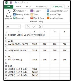
AND – returns TRUE if all conditions specified are true
Example: =AND (100<200, 200>100) TRUE because both conditions are true

OR – returns TRUE if at least one of the specified conditions is true
Example: =OR(100<200, 100>300) TRUE because one of the conditions is true

NOT – returns true if condition specified is NOT met (reverse logic)
Example: =NOT(100>500) TRUE because 100 is NOT greater than 500

XOR – also called Exclusive OR, returns true if either argument (but not both) is true
Examples:
=XOR(1+1=2, 2-1=2) returns TRUE because one condition is true and one is false
=XOR(1+1=2, 2-1=1) returns FALSE because both conditions are true
=XOR(5+1=2, 5-1=2) returns FALSE because both conditions are false

A few more things to note:
When you're searching for a range of results via Boolean operators, you define the range by what it's more than or less than. 
Excel 2013 allows a maximum of 255 arguments in a single logical function, but only if the formula does not exceed 8,192 characters.

Boolean operators may start out looking simple. When combined with other functions, however, such as IF statements, you can create some complex formulas that produce very powerful results.


Boolean AND, IF-AND

When you're trying to find something that meets multiple criteria, AND is your operator. For example: One of the actors in George’s play broke his leg, so George needs another actor, immediately, with very specific skills and appearance. In order to fit the costumes, the new guy must be 68 to 69 inches tall, must weigh between 180 and 200 pounds, and must be aged between 30 and 50.

If George’s list of actors contained only 50 to 100 names, he could scan the list and locate a replacement himself. But the Guild Actors database contains 20,000 records, so he needs a faster way to narrow the search.

For this query, you can use one of the following three formulas. All three formulas work and all are similar, except the AND statement only returns True or False. The IF statements allow custom responses such as “Match” or “Qualified.” 

Copy the database and formulas shown in figure 02 and experiment with the results.

A. AND statement using AND Boolean operators (with three conditions): returns true or false.

=AND(AND(C6>67,C6<70),AND(D6>179,D6<201),AND(E6>29,E6<51)) = TRUE

B. IF/AND statement using AND Boolean operators (with three conditions): returns Yes or No because the IF statement says: If this, and this, and this is true, then answer Yes; else/otherwise, answer No.

=IF(AND(AND(C8>67,C8<70),AND(D8>179,D8<201),AND(E8>29,E8<51)),”Yes”,”No”)

C. IF statement using AND Boolean operators (with three conditions): returns Yes or No.

In this case, if any of the AND statements are not met, the response will return False and the multiplication (asterisk) result will be 0 (False). This format often appears when your syntax has an error and Excel repairs it (after asking you if you would like assistance).

=IF(AND(C10>67,C10<70)*AND(D10>179,D10<201)*AND(E10>29,E10<51),”YES”,”NO”)

Note: Notice how Excel color-codes the formulas to the matching cells, including the opening and closing parentheses, in an effort to help you understand the syntax of each condition in the formula.

 02 Formulas that use AND, IF/AND, & IF statements.


Boolean OR, AND-OR

The first database search returned 1100 actors. George wants to narrow the results further, so he queries those 1100 results for two very specific skills: This actor must speak fluent Italian or French AND have a vocal range of tenor or bass. 

Use the following formula for this query:

=OR(OR(C9="Italian",C9="French"),AND(OR(D9="tenor",D9="base"))) = TRUE

Remember, for the answer to be true, the actor must speak Italian OR French AND sing tenor OR bass.

Any incorrect information produces a FALSE response.

Copy the database and formulas shown in figure 03 and experiment with the results. Once again, note how Excel color-codes the formulas to the matching cells, including the opening and closing parentheses, in an effort to help you understand the syntax of each condition in the formula.

03 Formula that uses OR, AND-OR operators


Boolean NOT, NOT-OR

The easiest way to explain the NOT operator is to compare it to an Internet search. If you searched online for your old friend Jack Russell just by typing his name, you'd get hundreds of hits for dogs and puppies, too. With the NOT operator, you can search for “Jack Russell NOT dogs NOT puppies” to remove the canine variable.

George needs some background performers to dance and play a variety of instruments—but not the piano, because pianists can't dance around, and not ballroom dancing, because he wants them to dance with their instruments, not with human partners. George queries the database again and specifies NOT piano AND NOT ballroom dancing.

Remember, this is reverse logic, so NOT piano and NOT ballroom equals FALSE because he doesn’t want ballroom and he doesn’t want piano. Think of FALSE as “No, not this person.” Notice also that record 3 (Feyd-Rautha) says guitar and ballroom. Guitar is good, but ballroom is bad, so the response is FALSE because George doesn’t want ballroom (even though guitar is okay). Same situation for record 4 (Piter De Vries), piano, waltz. Since only one is acceptable and not both, both are rejected.

Use the following formula for this query, then copy the database shown in figure 04 and experiment with the results.

=NOT(OR(C5="piano", D5="ballroom"))

04 Formula that uses NOT, NOT-OR operators


Meet XOR, also known as Exclusive OR

Just when you thought you had Boolean logic in the bag, Excel 2013 introduced the new operator XOR, which means Exclusive OR. Think of it as a similar opposite of NOT: If one condition is true and one is false, XOR returns TRUE. If both conditions are true, or both conditions are false, XOR returns FALSE.

Use the following formula for this query and then copy the database shown in figure 05 and experiment with the results.

=XOR(C5="piano", D5="ballroom")

05 Formula that uses XOR operator


Once you get comfortable with Boolean operators, you have a new skill for finding specific records in a sea of cells. Better yet, you can branch out to use Boolean logic to to refine Internet searches, database searches, and more. 

Read more on PCWorld.com...

Friday, March 25, 2016

Pivot Tables in Excel 2010

Pivot tables

A pivot table is essentially a dynamic summary report generated from a database. The database can reside in a worksheet (in the form of a table) or in an external data file. A pivot table can help transform endless rows and columns of numbers into a meaningful presentation of the data. Pivot table are very powerful tool for summarized analysis of the data.

Pivot tables are available under Insert tab » PivotTable dropdown » PivotTable

Pivot Table Example

Now let us see Pivot table with the help of example.Suppose you have huge data of voters and you want to see summarized data of voter Information per party then you can use Pivot table for it. Choose Insert tab » Pivot Table to insert pivot table. MS Excel selects the data of the table.You can select the pivot table location as existing sheet or new sheet.


This will generate the Pivot table pane as shown below.You have various options available in Pivot table pane as below. You can select fields for the generated pivot table.

  • Column labels : A field that has a column orientation in the pivot table. Each item in the field occupies a column.
  • Report Filter : You can set the filter for the report as year then data gets filtered as per the year.
  • Row labels: A field that has a row orientation in the pivot table. Each item in the field occupies a row.
  • Values area : The cells in a pivot table that contain the summary data. Excel offers several ways to summarize the data (sum, average, count, and so on).
After giving input fields to the pivot table, It will generate the pivot table with the data as below.


Read more on tutorialspoint.com...

Wednesday, March 23, 2016

Calculate Age or Working-period in a Format YY Years, MM Months, and DD Days.

In this posting, we will discuss how to calculate the age or working period with Excel in the format "YY Year, MM month, DD Day". So the output produced eg "20 Years, 6 Months, 12 Days."

Function DATEDIF
The main concept for calculating age or age working with Excel is comparing two dates, namely the date of birth or date of the first day of work with the current date. Excel functions or formulas to calculate the age or the age of the work that is DATEDIF (read: date dif) number of years, months and days between two dates is to use DATEDIF ().

Syntax:
DATEDIF (start_date, end_date, unit)
  • start_date is the earliest date in this case is the date of birth or date First Day of Work
  • end_date in this case, end date is the date that we can now replace with TODAY () or NOW ()
  • unit is the type of information required if the unit in the year (Y), month (M), day (D), Month in the same year (YM), or day of the same month (MD).

In this example, date of birth or date of the first day of work can be kept constant or fixed, while the Current Date or Date of First Working Day can be made relative to the function TODAY () or NOW (). The unit used for this purpose is Y Year YM MD Month and Day.

Excel formula to calculate the age or working-period in cell C6 is as follows:
=DATEDIF(B2,NOW(),"Y")&" years, "&DATEDIF(B2,NOW(),"YM")&" months, "&DATEDIF(B2,NOW(),"MD")&" days."

Results:

Sunday, March 20, 2016

Formula Errors

This chapter teaches you how to deal with some common formula errors in Excel.

##### error
When your cell contains this error code, the column isn't wide enough to display the value.

##### error

1. Click on the right border of the column A header and increase the column width.

Fix the ##### error


Tip: double click the right border of the column A header to automatically fit the widest cell in column A.

#NAME? error
The #NAME? error occurs when Excel does not recognize text in a formula.

#NAME? error

1. Simply correct SU to SUM.


#VALUE! error
Excel displays the #VALUE! error when a formula has the wrong type of argument.

#VALUE! error


1a. Change the value of cell A3 to a number.
1b. Use a function to ignore cells that contain text.

Fix the #VALUE! error


#DIV/0! error
Excel displays the #DIV/0! error when a formula tries to divide a number by 0 or an empty cell.

#DIV/0! error


1a. Change the value of cell A2 to a value that is not equal to 0.
1b. Prevent the error from being displayed by using the logical function IF.

Fix the #DIV/0! error


Explanation: if cell A2 equals 0, an empty string is displayed. If not, the result of the formula A1/A2 is displayed.

#REF! error
Excel displays the #REF! error when a formula refers to a cell that is not valid.

1. Cell C1 references cell A1 and cell B1.

#REF! Error Example

2. Delete column B. To achieve this, right click the column B header and click Delete.


3. Select cell B1. The reference to cell B1 is not valid anymore.

 #REF! Error Result

4. To fix this error, you can either delete +#REF! in the formula of cell B1 or you can undo your action by clicking Undo in the Quick Access Toolbar (or press CTRL + z).


Read more on excel-easy.com...

Array Formulas

This chapter helps you understand array formulas in Excel. Single cell array formulas perform multiple calculations in one cell.

Without Array Formula

Without using an array formula, we would execute the following steps to find the greatest progress.

1. First, we would calculate the progress of each student.


2. Next, we would use the MAX function to find the greatest progress.


With Array Formula

We don't need to store the range in column D. Excel can store this range in its memory. A range stored in Excel's memory is called an array constant.

1. We already know that we can find the progress of the first student by using the formula below.

With Excel Array Formula, Step 1


2. To find the greatest progress (don't be overwhelmed), we add the MAX function, replace C2 with C2:C6 and B2 with B2:B6.

With Excel Array Formula, Step 2


3. Finish by pressing CTRL + SHIFT + ENTER.

With Excel Array Formula, Step 3


Note: The formula bar indicates that this is an array formula by enclosing it in curly braces {}. Do not type these yourself. They will disappear when you edit the formula.

Explanation: The range (array constant) is stored in Excel's memory, not in an range. The array constant looks as follows:

{19;33;63;48;13}

This array constant is used as an argument for the MAX function, giving a result of 63.

F9 Key
When working with array formulas, you can have a look at these array constants yourself.

1. Select C2:C6-B2:B6 in the formula.

Select References


2. Press F9.

Array Constant


That looks good. Elements in a vertical array constant are separated by semicolons. Elements in a horizontal array constant are separated by commas.

Read more on excel-easy.com....

Saturday, March 19, 2016

Create a Macro

With Excel VBA you can automate tasks in Excel by writing so called macros. In this chapter, learn how to create a simple macro which will be executed after clicking on a command button. First, turn on the Developer tab.

Developer Tab
To turn on the Developter tab, execute the following steps.

1. Right click anywhere on the ribbon, and then click Customize the Ribbon.


2. Under Customize the Ribbon, on the right side of the dialog box, select Main tabs (if necessary).

3. Check the Developer check box.


4. Click OK.

5. You can find the Developer tab next to the View tab.


Command Button
To place a command button on your worksheet, execute the following steps.

1. On the Developer tab, click Insert.

2. In the ActiveX Controls group, click Command Button.


Assign a Macro
To assign a macro (one or more code lines) to the command button, execute the following steps.

1. Right click CommandButton1 (make sure Design Mode is selected).

2. Click View Code.


The Visual Basic Editor appears.

3. Place your cursor between Private Sub CommandButton1_Click() and End Sub.

4. Add the code line shown below.


Note: the window on the left with the names Sheet1, Sheet2 and Sheet3 is called the Project Explorer. If the Project Explorer is not visible, click View, Project Explorer. To add the Code window for the first sheet, click Sheet1 (Sheet1).

5. Close the Visual Basic Editor.

6. Click the command button on the sheet (make sure Design Mode is deselected).

Result:


Visual Basic Editor
To open the Visual Basic Editor, on the Developer tab, click Visual Basic.


The Visual Basic Editor appears.


Saturday, March 12, 2016

Simple Excel Timesheet

Simple Excel Timesheet


How to Create a Countdown Timer Clock in Excel and VBA

How to Create a Countdown Timer Clock in Excel and VBA


Here are 11 basic Excel tricks that will change your life

Microsoft Excel is an amazing piece of software, and even regular users might not be getting as much out of it as they can. Improve your Excel efficiency and proficiency with these basic shortcuts and functions that absolutely everyone needs to know.

1. Jump from worksheet to worksheet with Ctrl + PgDn and Ctrl + PgUp


2. Jump to the end of a data range or the next data range with Ctrl + Arrow
Of course you can move from cell to cell with arrow keys. But if you want to get around faster, hold down the Ctrl key and hit the arrow keys to get farther:


3. Add the Shift key to select data
Ctrl + Shift +Arrow will extend the current selection to the last nonblank cell in that direction:


4. Double click to copy down
To copy a formula or value down the length of your data set, you don’t need to hold and drag the mouse all the way down. Just double click the tiny box at the bottom right-hand corner of the cell:


5. Use shortcuts to quickly format values
For a number with two decimal points, use Ctrl + Shift + !. For dollars use Ctrl + Shift + $. For percentages it’s Ctrl + Shift + %. The last two should be pretty easy to remember:


6. Lock cells with F4
When copying formulas in Excel, sometimes you want your input cells to move with your formulas BUT SOMETIMES YOU DON’T. When you want to lock one of your inputs you need to put dollar signs before the column letter and row number. Typing in the dollar signs is insane and a huge waste of time. Instead, after you select your cell, hit F4 to insert the dollar signs and lock the cell. If you continue to hit the F4 key, it will cycle through different options: lock cell, lock row number, lock column letter, no lock.


7. Summarize data with CountIF and SumIF
CountIF will count the number of times a value appears in a selected range. The first input is the range of values you want to count in. The second input is the criteria, or particular value, you are looking for. Below we are counting the number of stories in column B written by the selected author:

COUNTIF(range,criteria)


SumIF will add up values in a range when the value in a corresponding range matches your criteria. Here we want to count the total number of views for each author. Our sum range is different from the range with the authors’ names, but the two ranges are the same size. We are adding up the number of views in column E when the author name in column B matches the selected name.

SUMIF(range,criteria,sum range)


8. Pull out the exact data you want with VLOOKUP
VLOOKUP looks for a value in the leftmost column of a data range and will return any value to the right of it. Here we have a list of law schools with school rankings in the first column. We want to use VLOOKUP to create a list of the top 5 ranked schools.

VLOOKUP(lookup value,data range,column number,type)

The first input is the lookup value. Here we use the ranking we want to find. The second input is the data range that contains the values we are looking up in the leftmost column and the information we’re trying to get in the columns to the right. The third input is the column number of the value you want to return.

We want the school name, and this is in the second column of our data range. The last input tells Excel if you want an exact match or an approximate match. For an exact match write FALSE or 0.


9. Use & to combine text strings
Here we have a column of first names and last names. We can create a column with full names by using &. In Excel, & joins together two or more pieces of text. Don’t forget to put a space between the names. Your formula will look like this =[First Name]&” “&[Last Name]. You can mix cell references with actual text as long as the text you want to include is surrounded by quotes:


10. Clean up text with LEFT, RIGHT and LEN
These text formulas are great for cleaning up data. Here we have state abbreviations combined with state names with a dash in between. We can use the LEFT function to return the state abbreviation. LEFT grabs a specified number of characters from the start of a text string. The first input is the text string. The second input is the number of characters you want. In our case, we want the first two characters:

LEFT(text string, number of characters)


If you want to pull the names of the states out of this text string you have to use the RIGHT function. RIGHT grabs a number of characters from the right end of a text string.

But how many characters on the right do you want? All but three, since the state names all come after the state’s two-letter abbreviation and a dash. This is where LEN comes in handy. LEN will count the number of characters or length of the text string.


Now you can use a combination of RIGHT and LEN to pull out the state names. Since we want all but the first three characters, we take the length of our string, subtract 3, and pull that many characters from the right end of the string:

RIGHT(text string,number of characters)


11. Generate random values with RAND
You can use RAND() function to generate a random value between 0 and 1. D0 not include any inputs, just leave the parentheses empty. New random values will be generated every time the workbook recalculates. You can force it to recalculate by hitting F9. But be careful. It also recalculates when you make other changes to the workbook:

RAND()


 The Video from Business Insider Excel


Read more at Business Insider