15 shortcuts that will be immediately useful for most users. This keyboard shortcut lists includes quick ways to format cells, navigate the program, and carry out a few operations.
The list is based on Excel 2016, but most will also work on Excel 2013. When that’s not the case we’ve noted it.
Keyboard access to the ribbon: Similar to the Vim-inspired add-ons for Chrome and Firefox, Excel 2013 and 2016 have a feature called Key Tips. When Key Tips appears by pressing Alt the Ribbon menu is overlaid with letters. Pressing a letter launches the corresponding menu item.
Ctrl + PgDn: Switch between worksheet tabs, moving left to right.
Ctrl + PgUp: Switch between worksheet tabs, moving right to left.
F12: Display the “Save As” dialog.
Ctrl + Shift + $: (Excel 2016) Current cell formatted as currency, with two decimal places and negative numbers in parentheses.
Ctrl + Shift + %: (Excel 2016) Current cell formatted as percentage with no decimal places.
Ctrl + Shift + #: (Excel 2016) Current cell formatted as date with day, month, year.
Ctrl + Shift + “:”: Insert current time.
Ctrl + Shift + “;”: Insert current date.
F4: Repeats the last command or action, if possible.
Shift + Arrow key: Extends your current cell selection by one addition cell in the direction specified.
Ctrl + F1: Display or hide the Ribbon.
Alt + Shift + F1: Insert a new worksheet tab.
Ctrl + F4: Close the current workbook.
Ctrl + D: Launches the Fill Down command for the selected cells below. Fill Down copies contents and format of the topmost cell in the column.
Microsoft Excel is an amazing piece of software, and even regular users might not be getting as much out of it as they can. Improve your Excel efficiency and proficiency with these basic shortcuts and functions that absolutely everyone needs to know.
1. Jump from worksheet to worksheet with Ctrl + PgDn and Ctrl + PgUp
2. Jump to the end of a data range or the next data range with Ctrl + Arrow
Of course you can move from cell to cell with arrow keys. But if you want to get around faster, hold down the Ctrl key and hit the arrow keys to get farther:
3. Add the Shift key to select data
Ctrl + Shift +Arrow will extend the current selection to the last nonblank cell in that direction:
4. Double click to copy down
To copy a formula or value down the length of your data set, you don’t need to hold and drag the mouse all the way down. Just double click the tiny box at the bottom right-hand corner of the cell:
5. Use shortcuts to quickly format values
For a number with two decimal points, use Ctrl + Shift + !. For dollars use Ctrl + Shift + $. For percentages it’s Ctrl + Shift + %. The last two should be pretty easy to remember:
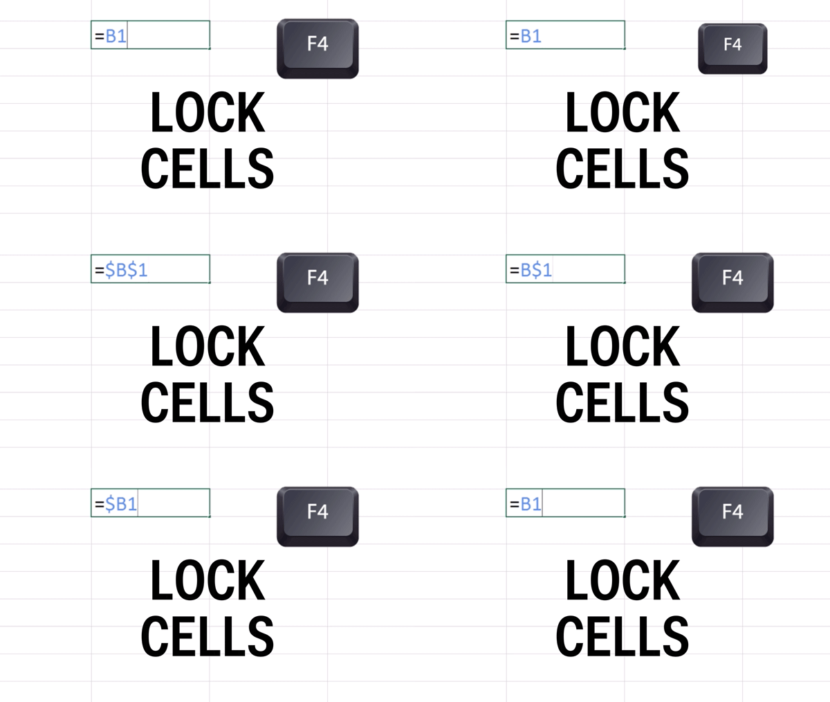
6. Lock cells with F4
When copying formulas in Excel, sometimes you want your input cells to move with your formulas BUT SOMETIMES YOU DON’T. When you want to lock one of your inputs you need to put dollar signs before the column letter and row number. Typing in the dollar signs is insane and a huge waste of time. Instead, after you select your cell, hit F4 to insert the dollar signs and lock the cell. If you continue to hit the F4 key, it will cycle through different options: lock cell, lock row number, lock column letter, no lock.
7. Summarize data with CountIF and SumIF
CountIF will count the number of times a value appears in a selected range. The first input is the range of values you want to count in. The second input is the criteria, or particular value, you are looking for. Below we are counting the number of stories in column B written by the selected author:
COUNTIF(range,criteria)
SumIF will add up values in a range when the value in a corresponding range matches your criteria. Here we want to count the total number of views for each author. Our sum range is different from the range with the authors’ names, but the two ranges are the same size. We are adding up the number of views in column E when the author name in column B matches the selected name.
SUMIF(range,criteria,sum range)
8. Pull out the exact data you want with VLOOKUP
VLOOKUP looks for a value in the leftmost column of a data range and will return any value to the right of it. Here we have a list of law schools with school rankings in the first column. We want to use VLOOKUP to create a list of the top 5 ranked schools.
The first input is the lookup value. Here we use the ranking we want to find. The second input is the data range that contains the values we are looking up in the leftmost column and the information we’re trying to get in the columns to the right. The third input is the column number of the value you want to return.
We want the school name, and this is in the second column of our data range. The last input tells Excel if you want an exact match or an approximate match. For an exact match write FALSE or 0.
9. Use & to combine text strings
Here we have a column of first names and last names. We can create a column with full names by using &. In Excel, & joins together two or more pieces of text. Don’t forget to put a space between the names. Your formula will look like this =[First Name]&” “&[Last Name]. You can mix cell references with actual text as long as the text you want to include is surrounded by quotes:
10. Clean up text with LEFT, RIGHT and LEN
These text formulas are great for cleaning up data. Here we have state abbreviations combined with state names with a dash in between. We can use the LEFT function to return the state abbreviation. LEFT grabs a specified number of characters from the start of a text string. The first input is the text string. The second input is the number of characters you want. In our case, we want the first two characters:
LEFT(text string, number of characters)
If you want to pull the names of the states out of this text string you have to use the RIGHT function. RIGHT grabs a number of characters from the right end of a text string.
But how many characters on the right do you want? All but three, since the state names all come after the state’s two-letter abbreviation and a dash. This is where LEN comes in handy. LEN will count the number of characters or length of the text string.
Now you can use a combination of RIGHT and LEN to pull out the state names. Since we want all but the first three characters, we take the length of our string, subtract 3, and pull that many characters from the right end of the string:
RIGHT(text string,number of characters)
11. Generate random values with RAND
You can use RAND() function to generate a random value between 0 and 1. D0 not include any inputs, just leave the parentheses empty. New random values will be generated every time the workbook recalculates. You can force it to recalculate by hitting F9. But be careful. It also recalculates when you make other changes to the workbook:
In this article you’ll learn, how to calculate number of days, weeks, months and years between 2 dates in Microsoft Excel.
To calculate the same, we’ll use INT, TODAY and MOD or we can use DATEDIF functions.
INT function, will get the whole number without decimal
MOD function, will divide the number by a divisor
TODAY function, will help us get the current date
DATEDIF function, will calculate difference between each pair of dates
Let’s take an example,
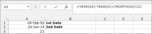
We have 2 dates,
Cell A1 containing 1st date and
Cell A2 containing 2nd date
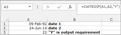
To calculate the difference between years, use DATEDIF function as shown in the following formula:
Select the cell A3 and write the formula =DATEDIF (A1,A2,”Y”)
This function will return the value in years
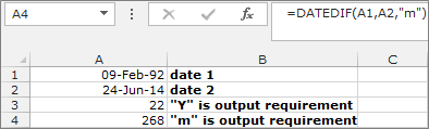
To calculate the difference in months, use the DATEDIF function as shown in the following formula:
Select the cell A4 and write the formula =DATEDIF (A1,A2,”M”)
This function will return the value in months
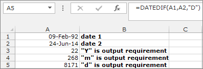
To calculate the difference between days, use the DATEDIF function as shown in the following formula:
Select the cell A5 and write the formula =DATEDIF (A1,A2,”D”)
This function will return the value in days
OR
Use the “YEAR”, “MONTH”, “AND” and “DAY” functions as shown in the following formula:-
Select the cell A3 and write the formula to calculate the years
=YEAR(A2)-YEAR(A1)-(MONTH(A2)/12)
This function will return the no. of years in between 2 dates
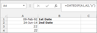
Use the DATEDIF function to calculate the number of days over years:-
Select the cell A4 and write the formula to calculate the years
=DATEDIF(A1,A2,”y”)
This function will return the no. of years in between 2 dates
PS: A lot of site, avoid calculating date in Excel using DATEDIF function. The reason is “bugs”. DATEDIF functions don’t have any documentation in Excel Help file.
But, Microsoft is continuously implying this feature / formula in all new version.
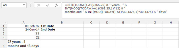
In case if you also want to avoid DATEDIF function, you can use manual calculation. Like below,
=INT((TODAY()-A1)/365.25) & ” years , ” & INT(MOD((TODAY()-A1)/365.25,1)*12) & ” months and ” & INT(MOD((TODAY()-A1)/30.4375,1)*30.4375) & ” days”.
It will give day difference in Year Month and in days. You can use A2 in case of today, where A2 is the greater day that A1 and gives you Elapsed time between these 2 dates.
If you are using Microsoft Excel in your daily life, you can use excel shortcuts to save time. While preparing any report or dashboard, if we use shortcut keys then the task would be completed in less time than expected.
Some of the best Excel shortcuts keys which are most essential are mentioned below. They will make the work of creating charts, formatting workbooks and analyzing data really easy and comfortable for the excel users.
In Excel we have so many shortcut keys in which few Excel key shortcuts we use regularly e.g. Ctrl+C is Excel copy shortcuts, Ctrl+V is Excel paste shortcuts etc.
Below are the few Excel 2010, Excel 2013 shortcuts keys
Tab
Moves one cell to the right in a worksheet
SHIFT+TAB
Moves to the previous cell in a worksheet.
CTRL+TAB
Switches to the next tab in dialog box.
CTRL+SHIFT+TAB
Switches to the previous tab in a dialog box.
CTRL+1
Displays the Format Cells dialog box.
CTRL+SHIFT+L
This is Excel filter keyboard shortcuts, use for filtering a column. E.g. If you have to set a couple of filters, and you already have filters placed in your data, instead of clearing each filter which is time-consuming, just turn-off and turn-on the filters, by pressing CTRL+SHIFT+L twice and your work is done.
CTRL+Arrow keys
To select a group of cells. Eg. it is difficult when you have to deal with large data and use the mouse to navigate the database. So to make your work easier, just rely on CTRL + arrow key combinations all the time to select a group of cells.
ALT+ES – Paste Special > Values
Pasting the value.E.g. When we apply any formula and want only the values to be shown in the cells, we need to use copy and then paste special values. If we need to get data from other workbooks or need to format existing tables, we can use ALT+ES (press E then leave the key and press S) to paste special value.
F4
Repeat the last command or action. E.g. If the color of text in a particular cell is changed, you can repeat the command by just pressing F4. This key can be used to repeat any action that was last performed provided the file is still open.
F2
Edit a selected cell. You can use F2 to edit a cell or formula in a cell.
Ctrl + F3
Add name for any range. E.g. If you are making a dashboard or Excel model, just press Shift + F3, no matter where you are (formula editing, conditional formatting, data validation etc.) and you get a list of all the defined names. Pick one and press ok to add it to the formula you are typing.
CTRL+K
Add Hyperlink. E.g. If you have more than a one sheet, Hyperlinks make your work book accessible and save your time. You can directly link the pages to one another using so that the sheets are accessible on a single click of the hyperlink.
CTRL+T –
Insert Table. E.g. If you have selected any cell in a range of related data just press CTRL+T to make it a table.
CTRL+S –
Save the sheet.
Ctrl + R
Fills the range to the right of the data
Ctrl + D
Fills range down word
Ctrl+W
Close a particular work book
F9
Refresh the sheets’ formula
Ctrl+PageDown/PageUp
Navigate sheets within the workbook
Ctrl+shift+1
Applies the Number format for two decimal places, thousands separator, and minus sign (-) for negative values.
Alt F11
Opens VBA editor
Ctrl F6
Switches to the next workbook window.
Ctrl ~
Change the cell value as general
Ctrl + spacebar
Select a particular column
Shift + spacebar
Select a particular row
Ctrl + Shift + spacebar
Select entire sheet
ALT + =
Auto sum for a column. E.g. When you have entered some data in a column and at the end of the column you need the summation of the column you can simply use ALT + = to save your time.
Ctrl + B
Applies and removes bold format.
F5
A Go-to window will open which allows you to go to a particular cell based on the reference provided.
Like VLOOKUP, the INDEX and MATCH functions pull in data from another dataset into one central location. Here are the main differences:
VLOOKUP is a much simpler formula. If you're working with large data sets that would require thousands of lookups, then using the INDEX MATCH function will significantly decrease load time in Excel.
INDEX MATCH formulas work right-to-left, whereas VLOOKUP formulas only work as a left-to-right lookup. In other words, if you need to do a lookup that has a lookup column to the right of the results column, then you'd have to rearrange those columns in order to do a VLOOKUP. This can be tedious with large datasets and/or lead to errors.
So if I want to combine information in Sheet 1 and Sheet 2 onto Sheet 1, but the column values in Sheets 1 and 2 aren't the same, then to do a VLOOKUP, I would need to switch around my columns. In this case, I'd choose to do an INDEX MATCH instead. Let's look at an example. Let's say Sheet 1 contains a list of people's names and their Hogwarts email addresses, and Sheet 2 contains a list of people's email addresses and the Patronus that each student has. (For the non-Harry Potter fans out there, every witch or wizard has an animal guardian called a "Patronus" associated with him or her.) The information that lives in both sheets is the column containing email addresses, but this email address column is in different column numbers on each sheet. I'd use the INDEX MATCH formula instead of VLOOKUP so I wouldn't have to switch any columns around. So what's the formula, then? The INDEX MATCH formula is actually the MATCH formula nested inside the INDEX formula. You'll see I differentiated the MATCH formula using a different color here. The formula: =INDEX(table array, MATCH formula) This becomes: =INDEX(table array, MATCH (lookup_value, lookup_array)) The formula with variables from our example below:=INDEX(Sheet2!A:A,(MATCH(Sheet1!C:C,Sheet2!C:C,0))) Here are the variables:
Table Array: The range of columns on Sheet 2 containing the new data you want to bring over to Sheet 1. In our example, "A" means Column A, which contains the "Patronus" information for each person.
Lookup Value: This is the column in Sheet 1 that contains identical values in both spreadsheets. In the example that follows, this means the "email" column on Sheet 1, which is Column C. So: Sheet1!C:C.
Lookup Array: This is the column in Sheet 2 that contains identical values in both spreadsheets. In the example that follows, this refers to the "email" column on Sheet 2, which happens to also be Column C. So: Sheet2!C:C.
Once you have your variables straight, type in the INDEX MATCH formula in the top-most cell of the blank Patronus column on Sheet 1, where you want the combined information to live
Instead of manually counting how often a certain value or number appears, let Excel do the work for you. With the COUNTIF function, Excel can count the number of times a word or number appears in any range of cells. For example, let's say I want to count the number of times the word "Gryffindor" appears in my data set. The formula: =COUNTIF(range, criteria) The formula with variables from our example below:=COUNTIF(D:D,"Gryffindor") In this formula, there are several variables:
Range: The range that we want the formula to cover. In this case, since we're only focusing on one column, we use "D:D" to indicate that the first and last column are both D. If I were looking at columns C and D, I would use "C:D."
Criteria: Whatever number or piece of text you want Excel to count. Only use quotation marks if you want the result to be text instead of a number. In our example, the criteria is "Gryffindor."
Simply typing in the COUNTIF formula in any cell and pressing "Enter" will show me how many times the word "Gryffindor" appears in the dataset.