This chapter helps you understand array formulas in Excel. Single cell array formulas perform multiple calculations in one cell.
Without Array Formula
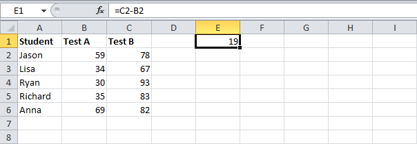
Without using an array formula, we would execute the following steps to find the greatest progress.
1. First, we would calculate the progress of each student.
2. Next, we would use the MAX function to find the greatest progress.
With Array Formula
We don't need to store the range in column D. Excel can store this range in its memory. A range stored in Excel's memory is called an array constant.
1. We already know that we can find the progress of the first student by using the formula below.
2. To find the greatest progress (don't be overwhelmed), we add the MAX function, replace C2 with C2:C6 and B2 with B2:B6.
3. Finish by pressing CTRL + SHIFT + ENTER.
Note: The formula bar indicates that this is an array formula by enclosing it in curly braces {}. Do not type these yourself. They will disappear when you edit the formula.
Explanation: The range (array constant) is stored in Excel's memory, not in an range. The array constant looks as follows:
{19;33;63;48;13}
This array constant is used as an argument for the MAX function, giving a result of 63.
F9 Key
When working with array formulas, you can have a look at these array constants yourself.
1. Select C2:C6-B2:B6 in the formula.
2. Press F9.
That looks good. Elements in a vertical array constant are separated by semicolons. Elements in a horizontal array constant are separated by commas.
With Excel VBA you can automate tasks in Excel by writing so called macros. In this chapter, learn how to create a simple macro which will be executed after clicking on a command button. First, turn on the Developer tab.
Developer Tab
To turn on the Developter tab, execute the following steps.
1. Right click anywhere on the ribbon, and then click Customize the Ribbon.
2. Under Customize the Ribbon, on the right side of the dialog box, select Main tabs (if necessary).
3. Check the Developer check box.
4. Click OK.
5. You can find the Developer tab next to the View tab.
Command Button
To place a command button on your worksheet, execute the following steps.
1. On the Developer tab, click Insert.
2. In the ActiveX Controls group, click Command Button.
Assign a Macro
To assign a macro (one or more code lines) to the command button, execute the following steps.
1. Right click CommandButton1 (make sure Design Mode is selected).
2. Click View Code.
The Visual Basic Editor appears.
3. Place your cursor between Private Sub CommandButton1_Click() and End Sub.
4. Add the code line shown below.
Note: the window on the left with the names Sheet1, Sheet2 and Sheet3 is called the Project Explorer. If the Project Explorer is not visible, click View, Project Explorer. To add the Code window for the first sheet, click Sheet1 (Sheet1).
5. Close the Visual Basic Editor.
6. Click the command button on the sheet (make sure Design Mode is deselected).
Result:
Visual Basic Editor
To open the Visual Basic Editor, on the Developer tab, click Visual Basic.
Microsoft Excel is an amazing piece of software, and even regular users might not be getting as much out of it as they can. Improve your Excel efficiency and proficiency with these basic shortcuts and functions that absolutely everyone needs to know.
1. Jump from worksheet to worksheet with Ctrl + PgDn and Ctrl + PgUp
2. Jump to the end of a data range or the next data range with Ctrl + Arrow
Of course you can move from cell to cell with arrow keys. But if you want to get around faster, hold down the Ctrl key and hit the arrow keys to get farther:
3. Add the Shift key to select data
Ctrl + Shift +Arrow will extend the current selection to the last nonblank cell in that direction:
4. Double click to copy down
To copy a formula or value down the length of your data set, you don’t need to hold and drag the mouse all the way down. Just double click the tiny box at the bottom right-hand corner of the cell:
5. Use shortcuts to quickly format values
For a number with two decimal points, use Ctrl + Shift + !. For dollars use Ctrl + Shift + $. For percentages it’s Ctrl + Shift + %. The last two should be pretty easy to remember:
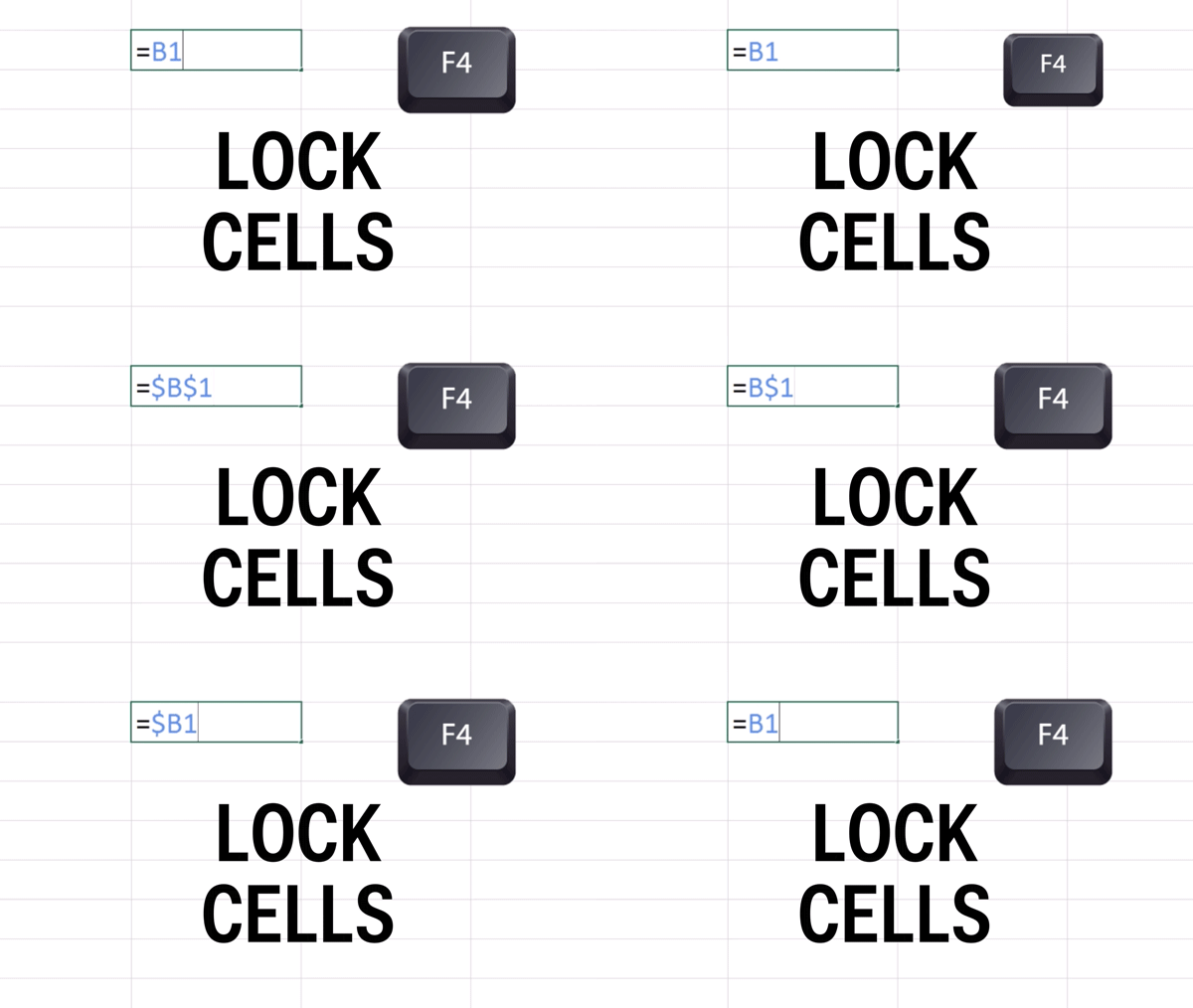
6. Lock cells with F4
When copying formulas in Excel, sometimes you want your input cells to move with your formulas BUT SOMETIMES YOU DON’T. When you want to lock one of your inputs you need to put dollar signs before the column letter and row number. Typing in the dollar signs is insane and a huge waste of time. Instead, after you select your cell, hit F4 to insert the dollar signs and lock the cell. If you continue to hit the F4 key, it will cycle through different options: lock cell, lock row number, lock column letter, no lock.
7. Summarize data with CountIF and SumIF
CountIF will count the number of times a value appears in a selected range. The first input is the range of values you want to count in. The second input is the criteria, or particular value, you are looking for. Below we are counting the number of stories in column B written by the selected author:
COUNTIF(range,criteria)
SumIF will add up values in a range when the value in a corresponding range matches your criteria. Here we want to count the total number of views for each author. Our sum range is different from the range with the authors’ names, but the two ranges are the same size. We are adding up the number of views in column E when the author name in column B matches the selected name.
SUMIF(range,criteria,sum range)
8. Pull out the exact data you want with VLOOKUP
VLOOKUP looks for a value in the leftmost column of a data range and will return any value to the right of it. Here we have a list of law schools with school rankings in the first column. We want to use VLOOKUP to create a list of the top 5 ranked schools.
The first input is the lookup value. Here we use the ranking we want to find. The second input is the data range that contains the values we are looking up in the leftmost column and the information we’re trying to get in the columns to the right. The third input is the column number of the value you want to return.
We want the school name, and this is in the second column of our data range. The last input tells Excel if you want an exact match or an approximate match. For an exact match write FALSE or 0.
9. Use & to combine text strings
Here we have a column of first names and last names. We can create a column with full names by using &. In Excel, & joins together two or more pieces of text. Don’t forget to put a space between the names. Your formula will look like this =[First Name]&” “&[Last Name]. You can mix cell references with actual text as long as the text you want to include is surrounded by quotes:
10. Clean up text with LEFT, RIGHT and LEN
These text formulas are great for cleaning up data. Here we have state abbreviations combined with state names with a dash in between. We can use the LEFT function to return the state abbreviation. LEFT grabs a specified number of characters from the start of a text string. The first input is the text string. The second input is the number of characters you want. In our case, we want the first two characters:
LEFT(text string, number of characters)
If you want to pull the names of the states out of this text string you have to use the RIGHT function. RIGHT grabs a number of characters from the right end of a text string.
But how many characters on the right do you want? All but three, since the state names all come after the state’s two-letter abbreviation and a dash. This is where LEN comes in handy. LEN will count the number of characters or length of the text string.
Now you can use a combination of RIGHT and LEN to pull out the state names. Since we want all but the first three characters, we take the length of our string, subtract 3, and pull that many characters from the right end of the string:
RIGHT(text string,number of characters)
11. Generate random values with RAND
You can use RAND() function to generate a random value between 0 and 1. D0 not include any inputs, just leave the parentheses empty. New random values will be generated every time the workbook recalculates. You can force it to recalculate by hitting F9. But be careful. It also recalculates when you make other changes to the workbook: