What-If Analysis - Scenario Manager

From excel-easy.com

What-If Analysis in Excel allows you to try out different values (scenarios) for formulas. The following example helps you master what-if analysis quickly and easily.

Assume you own a book store and have 100 books in storage. You sell a certain % for the highest price of $50 and a certain % for the lower price of $20.

If you sell 60% for the highest price, cell D10 calculates a total profit of 60 * $50 + 40 * $20 = $3800.

Create Different Scenarios

But what if you sell 70% for the highest price? And what if you sell 80% for the highest price? Or 90%, or even 100%? Each different percentage is a different scenario. You can use the Scenario Manager to create these scenarios.

Note: You can simply type in a different percentage into cell C4 to see the corresponding result of a scenario in cell D10. However, what-if analysis enables you to easily compare the results of different scenarios. Read on.

1. On the Data tab, click What-If Analysis and select Scenario Manager from the list.

​The Scenario Manager dialog box appears.

2. Add a scenario by clicking on Add.

3. Type a name (60% highest), select cell C4 (% sold for the highest price) for the Changing cells and click on OK.

4. Enter the corresponding value 0.6 and click on OK again.

5. Next, add 4 other scenarios (70%, 80%, 90% and 100%).

Finally, your Scenario Manager should be consistent with the picture below:

Note: to see the result of a scenario, select the scenario and click on the Show button. Excel will change the value of cell C4 accordingly for you to see the corresponding result on the sheet.

Scenario Summary

To easily compare the results of these scenarios, execute the following steps.

1. Click the Summary button in the Scenario Manager.

2. Next, select cell D10 (total profit) for the result cell and click on OK.

Result:

Conclusion: if you sell 70% for the highest price, you obtain a total profit of $4100, if you sell 80% for the highest price, you obtain a total profit of $4400, etc. That's how easy what-if analysis in Excel can be.

Step by Step Instructions for Easy EXCEL Dashboards

Step by Step Instructions for Easy EXCEL Dashboards
By David Wetton

x

Introduction to Pivot Tables, Charts, and Dashboards in Excel

By Jon Acampora of  ExcelCampus.com

Part 1
How to create an interactive dashboard using Pivot Tables and Pivot Charts.
Works with Excel 2003, 2007, 2010, 2013 for Windows & Excel 2011 for Mac

Download file used in the video



Part 2
In this video I explain some of the different pivot table calculation types. Learn how to calculate the average, count, sum, and percentage of total. I explain how to update your pivot table with more data, and also how to refresh your pivot tables.

The video contains a lot of Excel tips, like how to quickly make a duplicate copy of a sheet, how to select the visible cells only, and a lot of useful keyboard shortcuts.

Download file used in the video




Part 3
This is part 3 in the series on Pivot Tables and Dashboards. In this video we bring it all together to create the interactive dashboard.

You will learn how to:
- Group dates into months and years to create a time series trend chart.
- Group amounts to create a distribution (histogram) chart.
- Add slicers to your pivot tables and charts to make them interactive.
- Lots of tips and shortcuts for formatting your charts.

Download file used in the video

Built in Functions

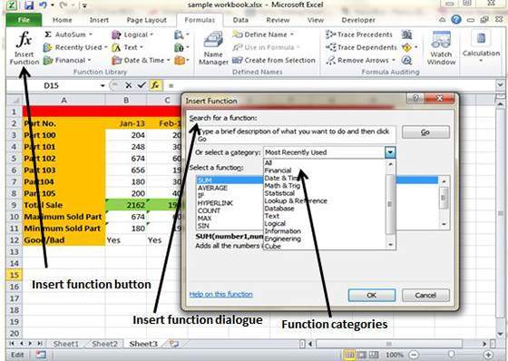
MS Excel has many built in functions which we can use in our formula. To see all the functions by category choose Formulas Tab » Insert Function. Then Insert function Dialog appears from which we can choose function.




Functions by categories
Let us see some of the built in functions in MS Excel.

Text Functions

• LOWER : Converts all characters in a supplied text string to lower case
• UPPER : Converts all characters in a supplied text string to upper case
• TRIM : Removes duplicate spaces, and spaces at the start and end of a text string
• CONCATENATE : Joins together two or more text strings
• LEFT : Returns a specified number of characters from the start of a supplied text string
• MID : Returns a specified number of characters from the middle of a supplied text string
• RIGHT : Returns a specified number of characters from the end of a supplied text string
• LEN : Returns the length of a supplied text string.
• FIND : Returns the position of a supplied character or text string from within a supplied text string (case-sensitive)

Date & Time

• DATE : Returns a date, from a user-supplied year, month and day
• TIME : Returns a time, from a user-supplied hour, minute and second
• DATEVALUE : Converts a text string showing a date, to an integer that represents the date in Excel's date-time code
• TIMEVALUE : Converts a text string showing a time, to a decimal that represents the time in Excel
• NOW : Returns the current date & time
• TODAY : Returns today's date

Statistical

• MAX : Returns the largest value from a list of supplied numbers
• MIN : Returns the smallest value from a list of supplied numbers
• AVERAGE : Returns the Average of a list of supplied numbers
• COUNT: Returns the number of numerical values in a supplied set of cells or values
• COUNTIF : Returns the number of cells (of a supplied range), that satisfy a given criteria
• SUM : Returns the sum of a supplied list of numbers

Logical

• AND : Tests a number of user-defined conditions and returns TRUE if ALL of the conditions evaluate to TRUE, or FALSE otherwise
• OR : Tests a number of user-defined conditions and returns TRUE if ANY of the conditions evaluate to TRUE, or FALSE otherwise
• NOT : Returns a logical value that is the opposite of a user supplied logical value or expression i.e. returns FALSE is the supplied argument is TRUE and returns TRUE if the supplied argument is FALSE)

Math & Trig

• ABS : Returns the absolute value (ie. the modulus) of a supplied number
• SIGN : Returns the sign (+1, -1 or 0) of a supplied number
• SQRT : Returns the positive square root of a given number
• MOD : Returns the remainder from a division between two supplied numbers

From tutorialspoint.com

Pivot Charts Excel 2010

Pivot Charts
A pivot chart is a graphical representation of a data summary displayed in a pivot table. A pivot chart is always based on a pivot table. Although Excel lets you create a pivot table and a pivot chart at the same time, you can’t create a pivot chart without a pivot table. All Excel charting features are available in a pivot chart

Pivot charts are available under Insert tab » PivotTable dropdown » PivotChart

Pivot Chart Example
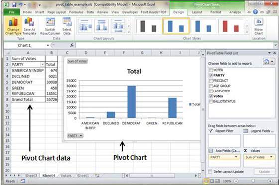
Now let us see Pivot table with the help of example. Suppose you have huge data of voters and you want to see summarized view of the data of voter Information per party in the form of charts then you can use Pivot chart for it. Choose Insert tab » Pivot Chart to insert pivot table.

MS Excel selects the data of the table.You can select the pivot chart location as existing sheet or new sheet. Pivot chart will depends on automatically created pivot table by the MS Excel. You can the the generated pivot chart in the below screen-shot



From TutorialsPoint.com...