How to Disable AutoFormatting on Import

Question:

How can I stop Microsoft Excel from auto formatting data when imported from a text file? Specifically, I want it to treat all of the values as text.

I am auditing insurance data in excel before it is uploaded to the new database. The files come to me as tab delimited text files. When loaded, Excel auto-formats the data causing leading 0's on Zip Codes, Routing Numbers and other codes, to be chopped off.

I don't have the patience to reformat all of the columns as text and guess how many zeros need to be replaced. Nor do I want to click through the import wizard an specify that each column is text.

Ideally I just want to turn off Excel's Auto-Formatting completely, and just edit every cell as it were plain text. I don't do any formula's or charts, just grid plain text editing.

Answer:
This should work for you: http://office.microsoft.com/en-us/excel-help/undo-or-turn-off-automatic-formatting-HA102491299.aspx#_Toc288715973

When Excel applies the automatic formatting, you can click the AutoCorrect Options button Button image that appears and choose to:

Undo the formatting (and you choose to redo it after you undo it) for this instance only

Change the specific AutoFormat options globally by clicking the stop option so that Excel stops making this change

Change the options for Excel by clicking Control AutoFormat Options.

How to disable specific Excel 2010 add-ins at startup?

Question:

I want to disable specific add-ins from loading in Excel 2010 every time I open up a new workbook or instance. How do I achieve this?

When I disable the specific add-ins by unchecking them in the normal Options menu, they still load when I open a new Excel.

Answer:

You can modify the LoadBehavior value in the registry for a particular Excel add-in to change its load behavior.

To modify the load behavior so the add-in is disabled when Excel opens, find the following path in registry:

HKEY_CURRENT_USER\Software\Microsoft\Office\Excel\Addins

All of your addins should be listed there. Click on a particular addin to see the registry values. A REG_DWORD value present in all of them is LoadBehavior and you can set it to disable automatic loading by right-clicking the LoadBehavior key > Modify... and entering a value of 0.

Here is a Microsoft link describing the other load behaviors: http://msdn.microsoft.com/en-us/library/bb386106.aspx#LoadBehavior

Calculating Number of Days, Weeks, Months and Years between Dates in Microsoft Excel

In this article you’ll learn, how to calculate number of days, weeks, months and years between 2 dates in Microsoft Excel.

To calculate the same, we’ll use INT, TODAY and MOD or we can use DATEDIF functions.

• INT function, will get the whole number without decimal
• MOD function, will divide the number by a divisor
• TODAY function, will help us get the current date
• DATEDIF function, will calculate difference between each pair of dates

Let’s take an example,

We have 2 dates,

• Cell A1 containing 1st date and
• Cell A2 containing 2nd date

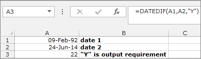
To calculate the difference between years, use DATEDIF function as shown in the following formula:

• Select the cell A3 and write the formula =DATEDIF (A1,A2,”Y”)
• This function will return the value in years

                        

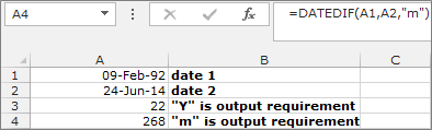
To calculate the difference in months, use the DATEDIF function as shown in the following formula:

• Select the cell A4 and write the formula =DATEDIF (A1,A2,”M”)
• This function will return the value in months

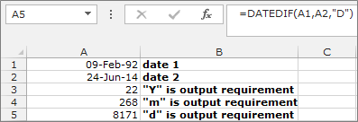
To calculate the difference between days, use the DATEDIF function as shown in the following formula:

• Select the cell A5 and write the formula =DATEDIF (A1,A2,”D”)
• This function will return the value in days

OR

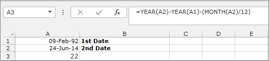
Use the “YEAR”, “MONTH”, “AND” and “DAY” functions as shown in the following formula:-

• Select the cell A3 and write the formula to calculate the years
• =YEAR(A2)-YEAR(A1)-(MONTH(A2)/12)
• This function will return the no. of years in between 2 dates

Use the DATEDIF function to calculate the number of days over years:-

• Select the cell A4 and write the formula to calculate the years
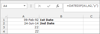
• =DATEDIF(A1,A2,”y”)
• This function will return the no. of years in between 2 dates

PS: A lot of site, avoid calculating date in Excel using DATEDIF function. The reason is “bugs”. DATEDIF functions don’t have any documentation in Excel Help file.

But, Microsoft is continuously implying this feature / formula in all new version.

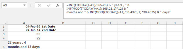
In case if you also want to avoid DATEDIF function, you can use manual calculation. Like below,

=INT((TODAY()-A1)/365.25) & ” years , ” & INT(MOD((TODAY()-A1)/365.25,1)*12) & ” months and ” & INT(MOD((TODAY()-A1)/30.4375,1)*30.4375) & ” days”.

It will give day difference in Year Month and in days. You can use A2 in case of today, where A2 is the greater day that A1 and gives you Elapsed time between these 2 dates.

Read more at exceltip.com:

http://www.exceltip.com/excel-date-time-formulas/calculating-number-of-days-weeks-months-and-years-between-dates.html

The Best Shortcut Keys in Microsoft Excel

If you are using Microsoft Excel in your daily life, you can use excel shortcuts to save time. While preparing any report or dashboard, if we use shortcut keys then the task would be completed in less time than expected.

Some of the best Excel shortcuts keys which are most essential are mentioned below. They will make the work of creating charts, formatting workbooks and analyzing data really easy and comfortable for the excel users.

In Excel we have so many shortcut keys in which few Excel key shortcuts we use regularly e.g. Ctrl+C is Excel copy shortcuts, Ctrl+V is Excel paste shortcuts etc.

Below are the few Excel 2010, Excel 2013 shortcuts keys

Tab	Moves one cell to the right in a worksheet
SHIFT+TAB	Moves to the previous cell in a worksheet.
CTRL+TAB	Switches to the next tab in dialog box.
CTRL+SHIFT+TAB	Switches to the previous tab in a dialog box.
CTRL+1	Displays the Format Cells dialog box.
CTRL+SHIFT+L	This is Excel filter keyboard shortcuts, use for filtering a column. E.g. If you have to set a couple of filters, and you already have filters placed in your data, instead of clearing each filter which is time-consuming, just turn-off and turn-on the filters, by pressing CTRL+SHIFT+L twice and your work is done.
CTRL+Arrow keys	To select a group of cells. Eg. it is difficult when you have to deal with large data and use the mouse to navigate the database.  So to make your work easier, just rely on CTRL + arrow key combinations all the time to select a group of cells.
ALT+ES – Paste Special > Values	Pasting the value.E.g. When we apply any formula and want only the values to be shown in the cells, we need to use copy and then paste special values. If we need to get data from other workbooks or need to format  existing tables, we can use ALT+ES (press E then leave the key and press S) to paste special value.
F4	Repeat the last command or action. E.g. If the color of text in a particular cell is changed, you can repeat the command by just pressing F4. This key can be used to repeat any action that was last performed provided the file is still open.
F2	Edit a selected cell. You can use F2 to edit a cell or formula in a cell.
Ctrl + F3	Add name for any range. E.g. If you are making a dashboard or Excel model, just press Shift + F3, no matter where you are (formula editing, conditional formatting, data validation etc.) and you get a list of all the defined names. Pick one and press ok to add it to the formula you are typing.
CTRL+K	Add Hyperlink. E.g. If you have more than a one sheet, Hyperlinks make your work book accessible and save your time. You can directly link the pages to one another using so that the sheets are accessible on a single click of the hyperlink.
CTRL+T –	Insert Table. E.g. If you have selected any cell in a range of related data just press CTRL+T to make it a table.
CTRL+S –	Save the sheet.
Ctrl + R	Fills the range to the right of the data
Ctrl + D	Fills range down word
Ctrl+W	Close a particular work book
F9	Refresh the sheets’ formula
Ctrl+PageDown/PageUp	Navigate sheets within the workbook
Ctrl+shift+1	Applies the Number format for two decimal places, thousands separator, and minus sign (-) for negative values.
Alt F11	Opens VBA editor
Ctrl F6	Switches to the next workbook window.
Ctrl ~	Change the cell value as general
Ctrl + spacebar	Select a particular column
Shift + spacebar	Select a particular row
Ctrl + Shift + spacebar	Select entire sheet
ALT + =	Auto sum for a column. E.g. When you have entered some data in a column and at the end of the column you need the summation of the column you can simply use ALT + = to save your time.
Ctrl + B	Applies and removes bold format.
F5	A Go-to window will open which allows you to go to a particular cell based on the reference provided. Applies the border of the cell.
Ctrl + Shift + &

Ref: http://www.exceltip.com/excel-keyboard-shortcuts/the-best-shortcut-keys-in-microsoft-excel.html

VLOOKUP Function

Have you ever had two sets of data on two different spreadsheets that you want to combine into a single spreadsheet?

For example, you might have a list of people's names next to their email addresses in one spreadsheet, and a list of those same people's email addresses next to their company names in the other -- but you want the names, email addresses, and company names of those people to appear in one place.

I have to combine data sets like this a lot -- and when I do, the VLOOKUP is my go-to formula. Before you use the formula, though, be absolutely sure that you have at least one column that appearsidentically in both places. Scour your data sets to make sure the column of data you're using to combine your information is exactly the same, including no extra spaces. 

The formula: =VLOOKUP(lookup value, table array, column number, [range lookup])

The formula with variables from our example below: =VLOOKUP(C2,Sheet2!A:B,2,FALSE)

In this formula, there are several variables. The following is true when you want to combine information in Sheet 1 and Sheet 2 onto Sheet 1.

• Lookup Value: This is the identical value you have in both spreadsheets. Choose the first value in your first spreadsheet. In the example that follows, this means the first email address on the list, or cell 2 (C2).
• Table Array: The range of columns on Sheet 2 you're going to pull your data from, including the column of data identical to your lookup value (in our example, email addresses) in Sheet 1 as well as the column of data you're trying to copy to Sheet 1. In our example, this is "Sheet2!A:B." "A" means Column A in Sheet 2, which is the column in Sheet 2 where the data identical to our lookup value (email) in Sheet 1 is listed. The "B" means Column B, which contains the information that's only available in Sheet 2 that you want to translate to Sheet 1.
• Column Number: If the table array (the range of columns you just indicated) this tells Excel which column the new data you want to copy to Sheet 1 is located in. In our example, this would be the column that "House" is located in. "House" is the second column in our range of columns (table array), so our column number is 2. [Note: Your range can be more than two columns. For example, if there are three columns on Sheet 2 -- Email, Age, and House -- and you still want to bring House onto Sheet 1, you can still use a VLOOKUP. You just need to change the "2" to a "3" so it pulls back the value in the third column: =VLOOKUP(C2:Sheet2!A:C,3,false).]
• Range Lookup: Use FALSE to ensure you pull in only exact value matches.

In the example below, Sheet 1 and Sheet 2 contain lists describing different information about the same people, and the common thread between the two is their email addresses. Let's say we want to combine both datasets so that all the house information from Sheet 2 translates over to Sheet 1.

So when we type in the formula =VLOOKUP(C2,Sheet2!A:B,2,FALSE), we bring all the house data into Sheet 1.

We've also written a full post about how to use the VLOOKUP function here (complete with video tutorial) if you still feel confused.

Keep in mind that VLOOKUP will only pull back values from the second sheet that are to the right of the column containing your identical data. This can lead to some limitations, which is why some people prefer to use the INDEX and MATCH functions instead.

Ref: http://blog.hubspot.com/marketing/how-to-use-excel-tips